KNN is the most intuitive classification algorithm you will study in Class 11. It does not build a complex model or learn equations — it simply remembers all the training data and classifies every new point by asking: “what do my nearest neighbours look like?” That simplicity is also what makes it powerful to understand. This guide covers the complete algorithm, step by step, exactly as your CBSE Unit 6 requires.
What You Will Learn
- What KNN is and how it classifies new data points
- The step-by-step process — from choosing K to making a prediction
- How Euclidean distance is calculated and why it matters
- Why the choice of K is critical — and how to think about it
- Python implementation using Scikit-learn (For Advanced Learners)
What Is KNN?
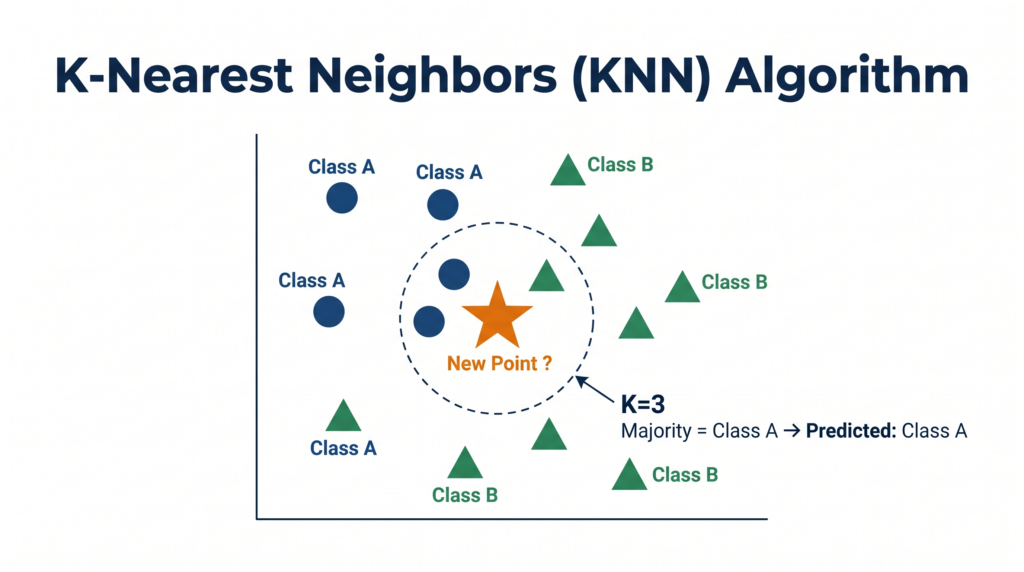
K-Nearest Neighbors (KNN) is a supervised machine learning algorithm used primarily for classification. It classifies a new, unknown data point by looking at the K most similar (nearest) data points already in the training dataset and assigning the class that the majority of those K neighbours belong to.
There is no training phase in the traditional sense — KNN stores all the training data and does all its work at prediction time. This makes it a lazy learner: it defers computation until a new point needs to be classified.
The core idea in one sentence: Tell me who your neighbours are, and I will tell you what you are.
📌 Class 11 Syllabus Note: KNN is covered under Unit 6 — Machine Learning Algorithms, under “Classification — How it works, Types, k-Nearest Neighbour algorithm.” Python implementation is marked “For Advanced Learners” and is not mandatory for the theory exam but is expected in practicals.
The KNN Algorithm — Step by Step
Given a new data point that needs to be classified, KNN follows exactly five steps every single time.
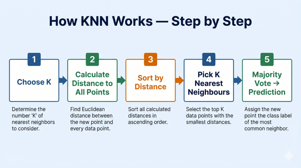
Step 1 — Choose the value of K
K is the number of nearest neighbours you will look at when classifying a new point. You choose K before running the algorithm.
- K = 3 means: look at the 3 closest training points
- K = 5 means: look at the 5 closest training points
- K must be a positive integer — typically an odd number to avoid tie votes
Choosing K is one of the most important decisions in KNN. We will cover this in detail shortly.
Step 2 — Calculate the distance from the new point to every training point
For every data point in your training set, calculate how far it is from the new point you want to classify. The standard distance metric used in KNN is Euclidean distance.
Euclidean Distance Formula:
For two points A = (x₁, y₁) and B = (x₂, y₂):
d = √[(x₂ – x₁)² + (y₂ – y₁)²]
This is simply the straight-line distance between two points in 2D space — the same formula from your Class 10 coordinate geometry, now applied to data features.
Worked example:
New point P = (3, 4). Training point Q = (6, 8).
d = √[(6-3)² + (8-4)²] d = √[3² + 4²] d = √[9 + 16] d = √25 d = 5
You repeat this calculation for every training point. The result is a list of distances from the new point to each existing point.
Step 3 — Sort all training points by distance (ascending)
Arrange all training data points from closest to furthest. The point with the smallest distance is at the top of the list.
Step 4 — Select the K nearest neighbours
Pick the top K entries from your sorted list. These are the K closest training points to the new data point you want to classify.
Step 5 — Majority vote → Final prediction
Look at the class labels of those K nearest neighbours. Whichever class appears most frequently among those K points is the predicted class for your new point.
Example: K = 5, neighbours are: Class A, Class A, Class B, Class A, Class B → Class A appears 3 times, Class B appears 2 times → Prediction: Class A (majority vote)
A Worked Example — Classifying a Fruit
Dataset: You have measurements of fruits: weight (grams) and diameter (cm), labelled as “Apple” or “Orange.”
| Fruit | Weight (g) | Diameter (cm) | Label |
|---|---|---|---|
| F1 | 150 | 7.0 | Apple |
| F2 | 170 | 7.5 | Apple |
| F3 | 130 | 6.5 | Apple |
| F4 | 200 | 8.5 | Orange |
| F5 | 210 | 8.8 | Orange |
| F6 | 190 | 8.2 | Orange |
New fruit to classify: Weight = 160g, Diameter = 7.2cm. K = 3.
Step 1: K = 3
Step 2: Calculate Euclidean distances from new point (160, 7.2) to each training point:
- d(F1) = √[(160-150)² + (7.2-7.0)²] = √[100 + 0.04] = √100.04 ≈ 10.0
- d(F2) = √[(160-170)² + (7.2-7.5)²] = √[100 + 0.09] = √100.09 ≈ 10.0
- d(F3) = √[(160-130)² + (7.2-6.5)²] = √[900 + 0.49] = √900.49 ≈ 30.0
- d(F4) = √[(160-200)² + (7.2-8.5)²] = √[1600 + 1.69] = √1601.69 ≈ 40.0
- d(F5) = √[(160-210)² + (7.2-8.8)²] = √[2500 + 2.56] = √2502.56 ≈ 50.0
- d(F6) = √[(160-190)² + (7.2-8.2)²] = √[900 + 1.0] = √901 ≈ 30.0
Step 3: Sort by distance: F1 (10.0), F2 (10.0), F3 (30.0), F6 (30.0), F4 (40.0), F5 (50.0)
Step 4: K = 3 nearest: F1 (Apple), F2 (Apple), F3 (Apple)
Step 5: Majority vote: Apple = 3, Orange = 0 → Prediction: Apple ✅
The new fruit with weight 160g and diameter 7.2cm is classified as an Apple.
Choosing K — Why It Matters Enormously
The value of K is a hyperparameter — you set it before training, and it directly controls the behaviour and accuracy of the model.
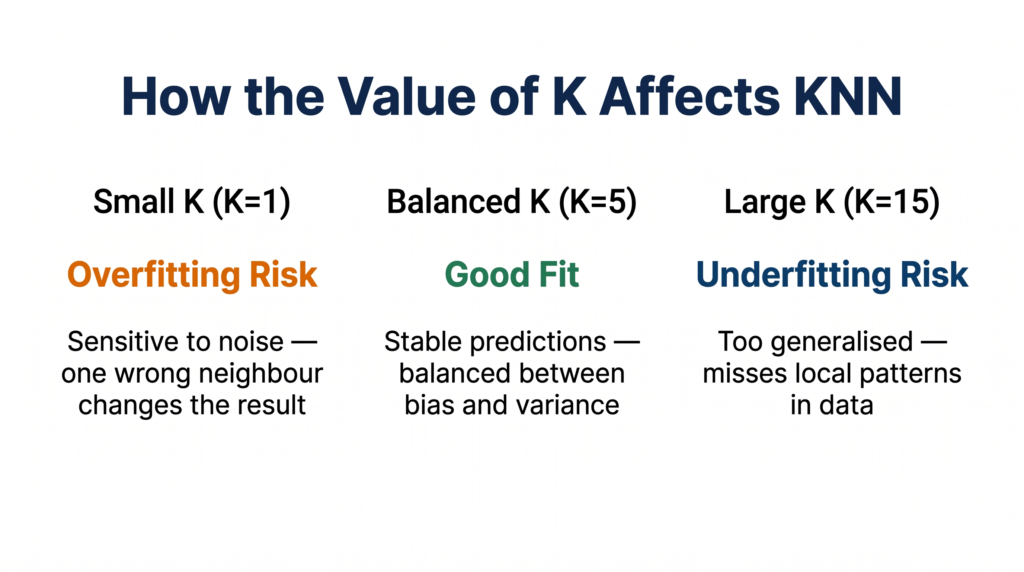
Small K (e.g., K = 1 or K = 3)
- The model is very sensitive to the training data
- A single noisy or mislabelled training point can swing the prediction
- The decision boundaries are jagged and irregular
- Risk: Overfitting — performs well on training data, poorly on new data
Large K (e.g., K = 15 or K = 20)
- The model considers too many neighbours, including distant ones
- It becomes overly generalised and starts ignoring local patterns
- Predictions become dominated by the majority class in the dataset
- Risk: Underfitting — too smooth, misses genuine local structure
Balanced K — The Goldilocks Zone
- Typically found by testing multiple values of K and measuring accuracy on a validation set
- Common starting point: K = √n where n is the number of training samples
- Always use an odd K for binary classification to avoid tie votes (e.g., use K = 5, not K = 4)
Rule of thumb for your exam: If asked why a specific K was chosen, the answer is: to balance between overfitting (too small K) and underfitting (too large K), tested using validation data.
KNN vs Linear Regression — Key Differences
Since both algorithms appear in your Class 11 Unit 6, exam questions sometimes ask you to compare them.
| Feature | KNN | Linear Regression |
|---|---|---|
| Task type | Classification (primarily) | Regression (predicts numbers) |
| Output | Class label (category) | Continuous numerical value |
| Training phase | None — lazy learner | Learns equation y = mx + c |
| Prediction method | Majority vote of K neighbours | Substitution into y = mx + c |
| Key parameter | K (number of neighbours) | m (slope) and c (intercept) |
| Interpretability | Moderate — can trace neighbours | High — equation is transparent |
| Sensitive to scale | Yes — feature scaling recommended | Less sensitive |
Python Implementation — KNN with Scikit-learn
⚠️ Note: Python implementation is marked “For Advanced Learners” in the CBSE 2025-26 Class 11 syllabus. Not mandatory for theory — but expected in practicals and IBM SkillsBuild.
python
# Program to demonstrate K-Nearest Neighbors (KNN) using Scikit-learn
# Dataset: Fruit classification based on weight and diameter

import numpy as np
from sklearn.neighbors import KNeighborsClassifier
from sklearn.preprocessing import StandardScaler

# Step 1: Training data — [weight, diameter]
X_train = np.array([
    [150, 7.0],   # Apple
    [170, 7.5],   # Apple
    [130, 6.5],   # Apple
    [200, 8.5],   # Orange
    [210, 8.8],   # Orange
    [190, 8.2]    # Orange
])
y_train = ['Apple', 'Apple', 'Apple', 'Orange', 'Orange', 'Orange']

# Step 2: Scale features (recommended for KNN — distance-based algorithm)
scaler = StandardScaler()
X_train_scaled = scaler.fit_transform(X_train)

# Step 3: Create and train the KNN model with K=3
k = 3
model = KNeighborsClassifier(n_neighbors=k)
model.fit(X_train_scaled, y_train)

# Step 4: Classify a new fruit — weight=160g, diameter=7.2cm
new_fruit = np.array([[160, 7.2]])
new_fruit_scaled = scaler.transform(new_fruit)
prediction = model.predict(new_fruit_scaled)

print(f"KNN Prediction (K={k}): {prediction[0]}")

# Step 5: Check what the 3 nearest neighbours are
distances, indices = model.kneighbors(new_fruit_scaled)
print(f"\n{k} Nearest Neighbours:")
for i, idx in enumerate(indices[0]):
    print(f"  Neighbour {i+1}: {y_train[idx]} (distance: {distances[0][i]:.3f})")
Expected Output:
KNN Prediction (K=3): Apple

3 Nearest Neighbours:
  Neighbour 1: Apple (distance: 0.231)
  Neighbour 2: Apple (distance: 0.284)
  Neighbour 3: Apple (distance: 1.847)
Key code notes:
StandardScaler()— scales all features to the same range before computing distances. Without scaling, a feature measured in grams (0–300) would dominate a feature measured in cm (5–10), making distances meaningless.KNeighborsClassifier(n_neighbors=3)— creates the KNN model with K=3model.kneighbors()— returns distances and indices of the K nearest neighbours, useful for understanding predictions- Scaled distances differ from our manual calculation above because scaling transforms the values before distance is computed
India Real-World Applications
Swiggy / Zomato — Restaurant Cuisine Classification: When a new restaurant registers on Swiggy, it is classified into a cuisine category (North Indian, South Indian, Chinese, etc.) by comparing its menu features to the K most similar restaurants already in the database. New restaurants with menu patterns closest to known South Indian restaurants get classified accordingly.
Healthcare — Patient Risk Grouping: Apollo Medics uses KNN-style systems to flag high-risk patients. A new patient’s age, BMI, blood pressure, and cholesterol readings are compared to thousands of past patients with known outcomes. The K most similar past patients determine whether the new patient is flagged as high-risk or low-risk.
Manufacturing — Quality Control: In a manufacturing line, sensor readings from each product unit (weight, dimensions, surface texture scores) are classified as “Pass” or “Fail” by comparing them to the K most similar units from historical production runs. This is KNN classification applied to industrial quality assurance — a direct application of the algorithm in operations like VCPL’s manufacturing environment.
Quick Revision Box
| Term | One-Line Definition |
|---|---|
| KNN | Supervised classification algorithm that predicts by majority vote of K nearest training points |
| K | The number of nearest neighbours to consider — a hyperparameter chosen before training |
| Euclidean Distance | Straight-line distance between two points: d = √[(x₂-x₁)² + (y₂-y₁)²] |
| Lazy Learner | An algorithm that stores all training data and defers computation to prediction time |
| Majority Vote | The final prediction step — whichever class appears most among the K neighbours wins |
| Hyperparameter | A setting chosen by the user before training (K in KNN, unlike parameters learned from data) |
| Feature Scaling | Normalising feature ranges before KNN so no single feature dominates distance calculations |
Practice Questions
Question 1 (2 marks): Explain how KNN classifies a new data point. What role does the value of K play?
Model Answer: KNN classifies a new data point by calculating its distance to every point in the training dataset, selecting the K closest points (nearest neighbours), and assigning the class that the majority of those K neighbours belong to.
The value of K controls how many neighbours influence the decision. A small K makes the model sensitive to individual data points (risk of overfitting), while a large K makes it overly generalised (risk of underfitting). The optimal K balances these two risks.
Question 2 (MCQ): In a KNN model with K=5, the 5 nearest neighbours of a new data point are: Class A, Class B, Class A, Class A, Class B. What is the predicted class?
(a) Class B — because it appears last (b) Class A — because it appears more frequently among the 5 neighbours (c) Cannot be determined without calculating distances again (d) Class B — because 2 is closer to 5 than 3
Answer: (b) Class A — because it appears more frequently among the 5 neighbours
Explanation: KNN prediction is decided by majority vote. Class A appears 3 times and Class B appears 2 times. Class A is the majority → predicted class is Class A. The distances have already been used to select these 5 neighbours — they are not recalculated at the voting step.
Frequently Asked Questions
Q1. Why does KNN need feature scaling but linear regression does not?
KNN is a distance-based algorithm — it calculates Euclidean distance between data points to find neighbours. If one feature is measured in thousands (e.g., salary in rupees: 30,000–80,000) and another in single digits (e.g., years of experience: 1–10), the salary feature will completely dominate the distance calculation, effectively making the experience feature irrelevant. Scaling (e.g., using StandardScaler) brings all features to a comparable range, so each feature contributes fairly to the distance. Linear regression uses an equation to find a line — distance between points is not computed, so scaling matters less.
Q2. What happens if there is a tie in the majority vote?
If K is even, ties are possible — for example, K=4 with 2 Class A and 2 Class B neighbours. Scikit-learn’s KNN breaks ties by prioritising the class that appears among the closer neighbours. To avoid this problem entirely, always choose an odd value of K for binary classification. This is a standard best practice, and mentioning it in a 4-mark answer on KNN demonstrates real understanding.
Q3. Is KNN only used for classification, or can it do regression too?
KNN can be used for both — KNeighborsClassifier for classification and KNeighborsRegressor for regression (available in Scikit-learn). For regression, instead of a majority vote, the algorithm takes the average of the K nearest neighbours’ output values as the prediction. However, the CBSE Class 11 syllabus covers KNN only as a classification algorithm. Regression in your syllabus is handled by Linear Regression. Knowing that a regression variant exists is useful context but is not required for your exam.