Linear regression is the first real machine learning algorithm you implement in Class 11 — and for good reason. It is the foundation of supervised learning, the starting point for understanding how machines learn from data, and directly examinable in your theory paper and practical. This guide walks you through everything: the concept, the formula, the Pearson correlation coefficient, the Excel demonstration, and the Python implementation.
What You Will Learn
- What linear regression is and what problem it solves
- The y = mx + c formula and what each term means in ML context
- What the Pearson correlation coefficient is and how to interpret it
- How to demonstrate linear regression in MS Excel (as required by your syllabus)
- Python code for linear regression using Scikit-learn (For Advanced Learners)
What Is Linear Regression?
Linear regression is a supervised learning algorithm used for regression tasks — it predicts a continuous numerical value as output.
Given a dataset of input-output pairs, linear regression finds the single straight line that best represents the relationship between the input (feature) and the output (target). Once this line is found, you can use it to predict the output for any new input value.
The core idea in one sentence: Find the straight line through the data that minimises the total prediction error.
Classic example for Class 11: Given data on how many hours students studied and what marks they scored, linear regression finds the line that best fits this pattern — and lets you predict what marks a student is likely to score if they study for, say, 6 hours.
📌 Class 11 Syllabus Note: Linear regression falls under Unit 6 — Machine Learning Algorithms. The CBSE 2025-26 curriculum covers: “Understanding Correlation, Regression, Finding the line, Linear Regression algorithm.” Practical requirements: calculation in MS-Excel and demonstration in Python (For Advanced Learners).
The Linear Regression Formula — y = mx + c
The mathematical equation for the best-fit line is:
y = mx + c
Where:
- y = the predicted output value (dependent variable) — e.g., marks scored
- x = the input feature (independent variable) — e.g., hours studied
- m = the slope of the line — how steeply it rises or falls; how much y changes for every 1-unit increase in x
- c = the intercept — the value of y when x = 0; where the line crosses the y-axis
Interpreting m and c with an example:
If your regression equation is y = 8x + 20 (where x = hours studied, y = marks):
- m = 8 means: for every additional hour of study, marks increase by 8 points
- c = 20 means: a student who studies 0 hours is still predicted to score 20 marks (baseline)
- To predict marks for 5 hours: y = 8(5) + 20 = 60 marks
This is the power of linear regression — once you have m and c, prediction is just substitution.
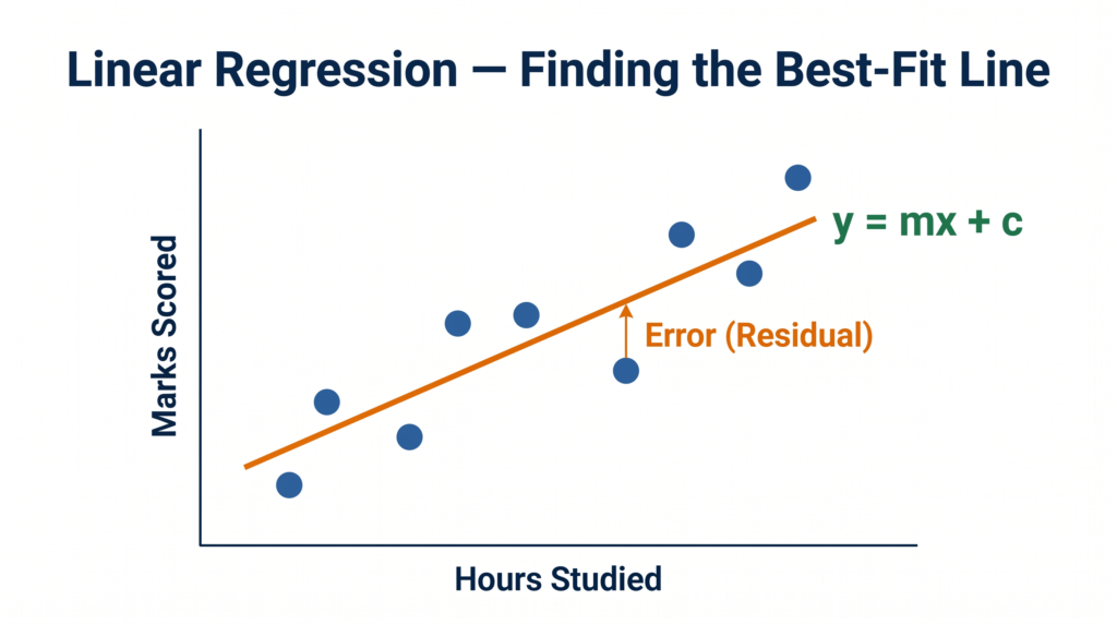
What does “best-fit” mean?
There are infinitely many lines you could draw through a scatter of data points. Linear regression finds the specific line that minimises the sum of squared errors (also called residuals) — the vertical distances between each actual data point and the predicted line. This optimisation process is called the Ordinary Least Squares (OLS) method.
For your exam, you do not need to derive the formula for m and c manually — but understanding what “best-fit” means (minimises total error) is important for 4-mark answers.
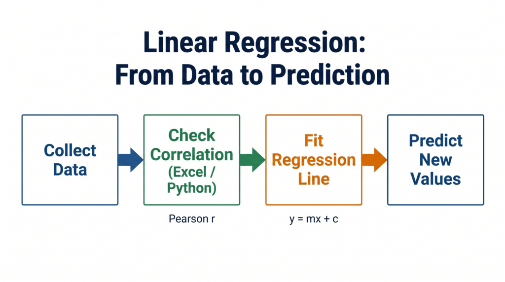
Step 1 Before Regression — Pearson Correlation Coefficient
Before applying linear regression, you must first check whether a linear relationship between the two variables actually exists. This is done using the Pearson Correlation Coefficient, denoted by r.
Definition: The Pearson correlation coefficient measures the strength and direction of the linear relationship between two variables. It always falls between -1 and +1.
Interpreting the value of r
| Value of r | Interpretation |
|---|---|
| r = +1 | Perfect positive correlation — as x increases, y increases proportionally |
| 0.7 ≤ r < 1 | Strong positive correlation |
| 0.3 ≤ r < 0.7 | Moderate positive correlation |
| r ≈ 0 | No linear correlation — linear regression would not be meaningful |
| -0.3 > r ≥ -0.7 | Moderate negative correlation |
| -0.7 > r ≥ -1 | Strong negative correlation |
| r = -1 | Perfect negative correlation — as x increases, y decreases proportionally |
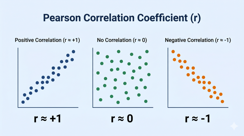
What does each type look like?
Positive correlation (r close to +1): Hours studied vs marks scored — as study hours go up, marks tend to go up. Points on a scatter plot trend upward from left to right.
No correlation (r close to 0): Shoe size vs marks scored — no meaningful relationship. Points scattered randomly.
Negative correlation (r close to -1): Hours of sleep lost vs exam performance — as sleep decreases, performance tends to decrease too. Points trend downward from left to right.
Rule for applying linear regression
If |r| < 0.3 (close to zero), a linear relationship is too weak — linear regression is not a reliable model for that data. Always check correlation before fitting a line.
📌 Class 11 Exam Note: The CBSE 2025-26 syllabus explicitly includes “Calculation of Pearson correlation coefficient in MS-Excel” as a practical requirement. Know the interpretation ranges and be able to state whether regression is appropriate based on the r value.
Demonstrating Linear Regression in MS Excel
The CBSE Class 11 syllabus requires you to demonstrate linear regression in MS Excel. Here is the step-by-step process:
Dataset — Hours Studied vs Marks Scored:
| Hours Studied (x) | Marks Scored (y) |
|---|---|
| 1 | 25 |
| 2 | 35 |
| 3 | 45 |
| 4 | 50 |
| 5 | 60 |
| 6 | 70 |
| 7 | 75 |
Step 1 — Enter data in Excel. Put Hours Studied in Column A and Marks Scored in Column B.
Step 2 — Calculate Pearson correlation coefficient. In an empty cell, type: =CORREL(A2:A8, B2:B8) This gives the r value. For this data, r ≈ 0.99 — strong positive correlation, so linear regression is appropriate.
Step 3 — Create a Scatter Plot. Select both columns → Insert → Chart → Scatter (X, Y).
Step 4 — Add a Trendline (Regression Line). Click on any data point in the chart → Right-click → “Add Trendline” → Select “Linear” → Check “Display Equation on chart” and “Display R-squared value.”
Step 5 — Read the equation. Excel displays the equation in the form y = mx + c directly on the chart. For this data, it will be approximately y = 8.5x + 17.1.
Step 6 — Make a prediction. To predict marks for 8 hours of study: y = 8.5(8) + 17.1 = 85.1 marks
This complete Excel workflow is what your practical exam tests. Practice it until you can do it without notes.
Python Implementation — Linear Regression with Scikit-learn
⚠️ Note for Class 11 students: Python implementation of linear regression is marked “For Advanced Learners” in the CBSE 2025-26 syllabus. It is not mandatory for your theory exam but is highly valuable for your practical file and IBM SkillsBuild assessment.
python
# Program to demonstrate Linear Regression using Scikit-learn
# Dataset: Hours Studied vs Marks Scored

import numpy as np
import matplotlib.pyplot as plt
from sklearn.linear_model import LinearRegression

# Step 1: Prepare the data
hours = np.array([1, 2, 3, 4, 5, 6, 7]).reshape(-1, 1)  # Input (X) - must be 2D
marks = np.array([25, 35, 45, 50, 60, 70, 75])           # Output (y)

# Step 2: Create and train the model
model = LinearRegression()
model.fit(hours, marks)

# Step 3: View the equation parameters
print(f"Slope (m): {model.coef_[0]:.2f}")
print(f"Intercept (c): {model.intercept_:.2f}")
print(f"Equation: y = {model.coef_[0]:.2f}x + {model.intercept_:.2f}")

# Step 4: Make a prediction
hours_to_predict = np.array([[8]])
predicted_marks = model.predict(hours_to_predict)
print(f"Predicted marks for 8 hours: {predicted_marks[0]:.1f}")

# Step 5: Plot the results
plt.scatter(hours, marks, color='#1A3A6B', label='Actual Data')
plt.plot(hours, model.predict(hours), color='#E8710A', label='Regression Line')
plt.xlabel('Hours Studied')
plt.ylabel('Marks Scored')
plt.title('Linear Regression: Hours Studied vs Marks Scored')
plt.legend()
plt.grid(True)
plt.show()
Expected Output:
Slope (m): 8.57
Intercept (c): 16.43
Equation: y = 8.57x + 16.43
Predicted marks for 8 hours: 85.0
Line-by-line explanation:
reshape(-1, 1)— Scikit-learn requires the input X to be a 2D array (column vector), not a flat listLinearRegression()— creates the model object.fit(hours, marks)— this is where learning happens; the model calculates the best m and cmodel.coef_[0]— gives the slope mmodel.intercept_— gives the y-intercept cmodel.predict()— uses the learned equation to predict for new input valuesplt.scatter()+plt.plot()— plots the original data points and the fitted line together
India Real-World Applications
Manufacturing — Predicting Machine Downtime (VCPL-style application): In a manufacturing plant, engineers track machine operating temperature (°C) against downtime hours per month. Linear regression fits a line to this data. Once the equation is known — say y = 0.8x – 20 — a reading of 60°C predicts 28 hours of downtime next month, prompting early maintenance scheduling. This is regression predicting a continuous number (downtime hours) from a continuous input (temperature).
Agriculture — Fertiliser vs Crop Yield: ICAR (Indian Council of Agricultural Research) uses linear regression to model the relationship between fertiliser quantity (kg per hectare) and crop yield (tonnes per hectare) across different soil types. Farmers in Punjab use these equations to optimise inputs and reduce costs.
Education — Board Marks Prediction: Coaching institutes use linear regression models built on past student data (mock test scores, attendance) to predict individual students’ likely board scores. Schools use these predictions to identify students needing additional support before the exams.
Quick Revision Box
| Term | One-Line Definition |
|---|---|
| Linear Regression | Supervised ML algorithm that finds the best-fit straight line to predict a numerical output |
| Best-Fit Line | The line that minimises the total squared error between predicted and actual values |
| y = mx + c | The regression equation — y is predicted output, x is input, m is slope, c is intercept |
| Slope (m) | How much y changes for every 1-unit increase in x |
| Intercept (c) | The value of y when x = 0 — where the line crosses the y-axis |
| Pearson r | Measures strength and direction of linear relationship between two variables (-1 to +1) |
| Positive Correlation | As x increases, y increases — r is positive and close to +1 |
| Negative Correlation | As x increases, y decreases — r is negative and close to -1 |
| Residual / Error | The vertical distance between an actual data point and the predicted line |
Practice Questions
Question 1 (2 marks): What is the Pearson correlation coefficient? What does a value of r = -0.9 indicate?
Model Answer: The Pearson correlation coefficient (r) measures the strength and direction of the linear relationship between two variables. Its value always falls between -1 and +1.
A value of r = -0.9 indicates a strong negative correlation — as one variable increases, the other decreases strongly and consistently. This means linear regression would be a good fit for this data, and the regression line would slope downward from left to right.
Question 2 (MCQ): A student uses linear regression to predict delivery time (in minutes) for a food delivery app based on distance (in km). The equation obtained is y = 4x + 5. What is the predicted delivery time for a distance of 8 km?
(a) 32 minutes (b) 37 minutes (c) 45 minutes (d) 20 minutes
Answer: (b) 37 minutes
Explanation: Substitute x = 8 into y = 4x + 5: y = 4(8) + 5 = 32 + 5 = 37 minutes
Option (a) forgets to add the intercept c = 5. Always substitute the complete equation including both m and c.
Frequently Asked Questions
Q1. Can linear regression predict values outside the range of training data?
Technically yes — the equation y = mx + c can be evaluated for any x value. But doing so is risky. When you predict for x values far beyond your training data range, the reliability drops significantly because you are assuming the linear pattern continues indefinitely. This is called extrapolation, as opposed to interpolation (predicting within the training range). For your Class 11 exam, stick to predictions within or close to your data range unless the question specifically asks about extrapolation.
Q2. What is the difference between r (Pearson correlation) and R² (R-squared)?
r measures the direction and strength of the linear relationship. R² (r squared) measures the proportion of variance in y that is explained by x — essentially, how well the regression line fits the data. An R² of 0.95 means 95% of the variation in marks scored is explained by hours studied. Excel displays R² automatically when you add a trendline. For most Class 11 questions, understanding r is sufficient — R² is good extra knowledge if you see it in Excel output.
Q3. Why must X be reshaped to 2D in the Python Scikit-learn code?
Scikit-learn’s fit() method expects the input X to be a 2D array (like a table with rows and columns) because in real ML problems, you usually have multiple input features, not just one. Each row is one data point and each column is one feature. Even when you have a single feature like hours studied, Scikit-learn still expects it formatted as a column — which is what .reshape(-1, 1) does: it converts a flat list like [1, 2, 3] into a column like [[1], [2], [3]]. Forgetting this reshape is one of the most common errors beginners make.